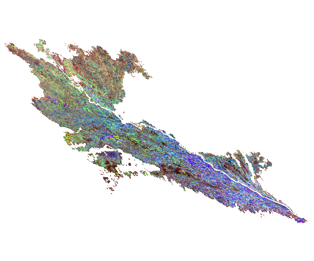
We are going to classify a multitemporal image stack of MODIS NDVI time series (MOD13Q1). The stack consists of 23 bands (16-day composites) with a spatial resolution of 231m in sinusoidal projection. We want to classify the different land use types, especially to discriminate different crop types.

Install Python and required image processing and scientific programming packages:

sudo apt-get install python-numpy scikit-learn scikit-image

For beginners, the basic Python IDLE is sufficient for scripting. However, another IDE, LiClipse is highly recommended: http://www.liclipse.com/

We assume that you already have created a bunch of training samples in 8bit TIFF format with distinct class labeling (1,2,3,4, etc). It is necessary that these single pixels are snapped to the pixel size of the original dataset and have the same dimensions and extent.

Now write your Training script:

# import all required Python packages:
import skimage.io as io
import numpy as np
import os, shutil
   
from sklearn.ensemble import AdaBoostClassifier, RandomForestClassifier, GradientBoostingClassifier, ExtraTreesClassifier
from sklearn.externals import joblib

# set up your directories with the MODIS data
 rootdir = "C:\\Data\\Raster\\MODIS\\"
# path to your training data
path_pix = "C:\\Data\\Samples\\"
# path to your model
path_model = "C:\\Data\\Models\\"
# path to your classification results
path_class = "C:\\Data\\Class\\"

 # declare a new function
 def training():
    # path to your MODIS TIFF  
    raster = rootdir + "modis_stack_ndvi.tif"
    # path to your corresponding pixel samples (training data) 
    samples = path_pix + "samples_modis.tif"  

    # read in MODIS raster
    img_ds = io.imread(raster)
    # convert to 16bit numpy array 
    img = np.array(img_ds, dtype='int16')

    # do the same with your sample pixels 
    roi_ds = io.imread(samples)   
    roi = np.array(roi_ds, dtype='int8')  
    
    # read in your labels
    labels = np.unique(roi[roi > 0]) 
    print('The training data include {n} classes: {classes}'.format(n=labels.size, classes=labels))

    # compose your X,Y data (dataset - training data)     
    X = img[roi > 0, :] 
    Y = roi[roi > 0]     

    # assign class weights (class 1 has the weight 3, etc.)
    weights = {1:3, 2:2, 3:2, 4:2}

    # build your Random Forest Classifier 
    # for more information: http://scikit-learn.org/stable/modules/generated/sklearn.ensemble.RandomForestClassifier.html

    rf = RandomForestClassifier(class_weight = weights, n_estimators = 100, criterion = 'gini', max_depth = 4, 
                                min_samples_split = 2, min_samples_leaf = 1, max_features = 'auto', 
                                bootstrap = True, oob_score = True, n_jobs = 1, random_state = None, verbose = True)  

    # alternatively you may try out a Gradient Boosting Classifier 
    # It is much less RAM consuming and considers weak training data      
    """ 
    rf = GradientBoostingClassifier(n_estimators = 300, min_samples_leaf = 1, min_samples_split = 4, max_depth = 4,    
                                    max_features = 'auto', learning_rate = 0.8, subsample = 1, random_state = None,         
                                    warm_start = True)
    """

    # now fit your training data with the original dataset
    rf = rf.fit(X,Y)

    # export your Random Forest / Gradient Boosting Model     
    model = path_model + "model.pkl"
    joblib.dump(rf, model)

training()

And now write your classification script:

def classification():
    # Read worldfile of original dataset
    tfw_old = str(raster.split(".tif")[0]) + ".tfw"     

    # Read Data    
    img_ds = io.imread(raster)   
    img = np.array(img_ds, dtype='int16')    

    # call your random forest model
    rf = path_model + "model.pkl"          
    clf = joblib.load(rf)    

    # Classification of array and save as image (23 refers to the number of multitemporal NDVI bands in the stack) 
    new_shape = (img.shape[0] * img.shape[1], img.shape[2]) 
    img_as_array = img[:, :, :23].reshape(new_shape)   

    class_prediction = clf.predict(img_as_array) 
    class_prediction = class_prediction.reshape(img[:, :, 0].shape)  

    # now export your classificaiton
    classification = path_class  + "classification.tif" 
    io.imsave(classification, class_prediction)    

    # Assign Worldfile to classified image    
    tfw_new = classification.split(".tif")[0] + ".tfw"   
    shutil.copy(tfw_old, tfw_new)

classification()

Multitemporal NDVI MODIS Stack with clipped AOI:

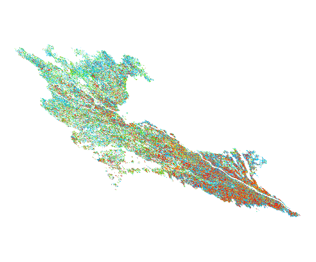
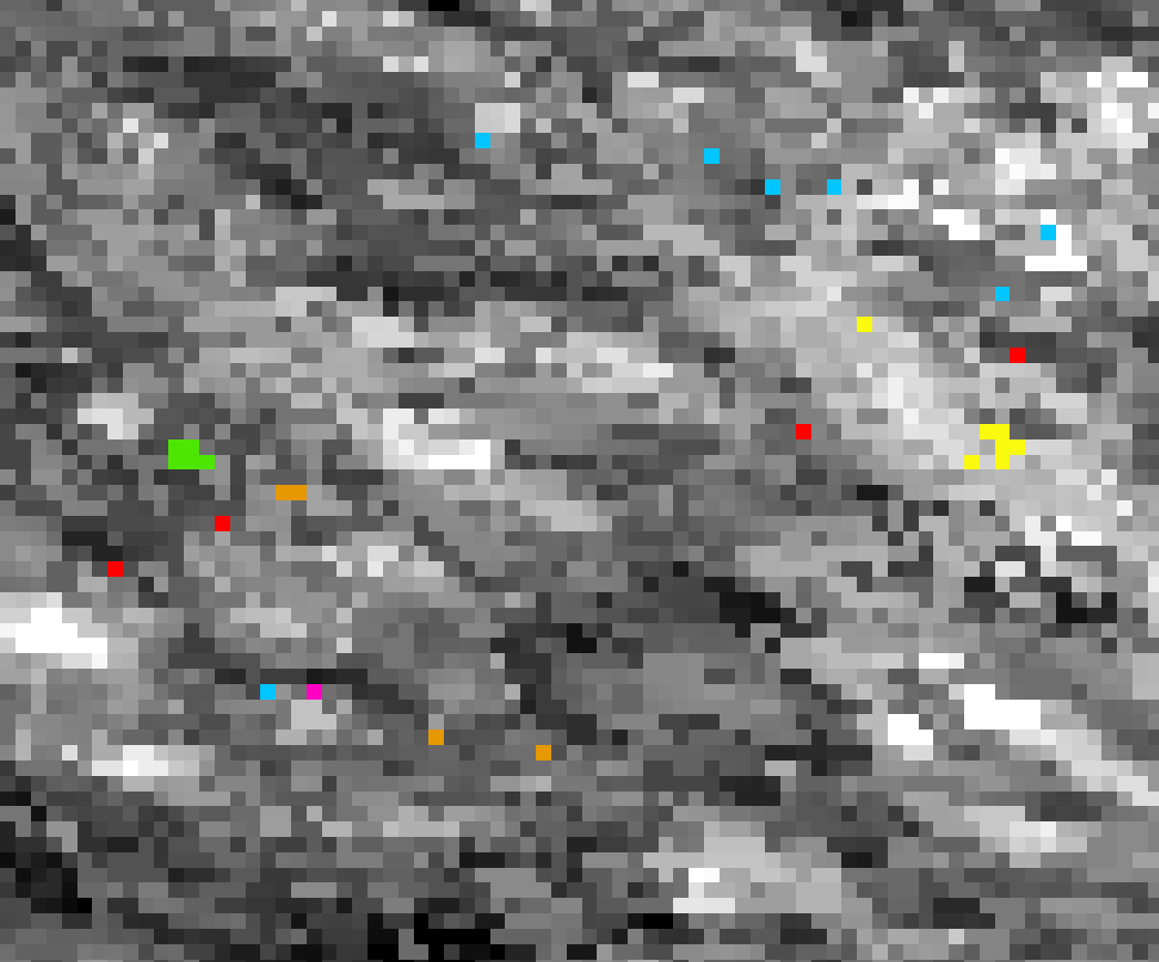
Training pixels with distinct classes are created from field sampling points and snapped to the original raster extent:

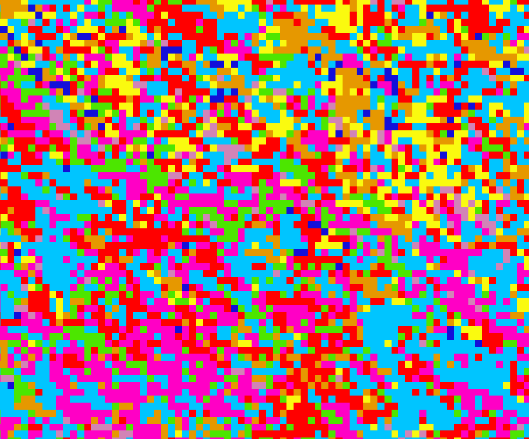
Classification results (left image: same extent as above):